PyTorch Playground
a little-more-than-introductory guide to help people get comfortable with PyTorch functionalities


- Dataset and Transforms
- Writing Custom Autograd Functions / Layers
- Basic Training and Validation Loop
- Tensorboard
- Inference
- Saving and Loading Models
- Extra Resources
![]()
Dataset and Transforms
- Dataset Class : manages the data, labels and data augmentations
- DataLoader Class : manages the size of the minibatch
Creating your Own Dataset
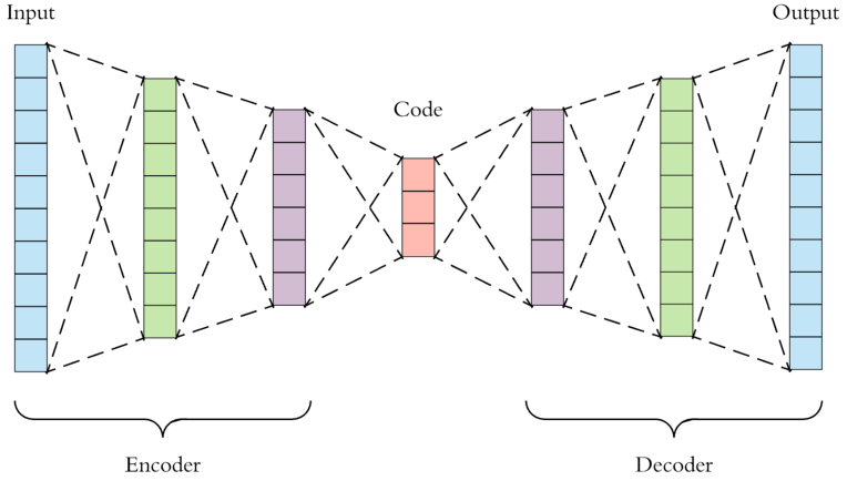
Let's take the example of training an autoencoder in which our training data only consists of images.
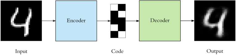
The encoder can be made up of convolutional or linear layers.
To create our own dataset class in PyTorch we inherit from the torch.utils.data.Dataset class and define two main methods, the __len__ and the __getitem__
from torch.utils.data import Dataset
from torchvision import transforms
from PIL import Image
from typing import List

class ImageDataset(Dataset):
    """
    A class for creating data and augemntation pipeline
    """
    def __init__(self, glob_pattern:str, patchsize:int):
        """
        Parameters
        ----------
        glob_pattern: this pattern must expand
            to a list of RGB images in PNG format.
            For eg. "/data/train/cat/*.png"

        patchsize: the size you want to crop
            the image to

        """
        self.image_paths_list = glob.glob(glob_pattern)
        self.patchsize = patchsize

    def __len__(self):
        # denotes size of data
        return len(self.image_paths_list)

    def transform(self, image):
        # convert to RGB if image is B/W
        if image.mode == 'L':
            image = image.convert('RGB')
        self.data_transforms = transforms.Compose([transforms.RandomCrop(size = self.patchsize),
                                                   transforms.RandomHorizontalFlip(),
                                                   transforms.RandomVerticalFlip(),
                                                   transforms.ToTensor()])
        return self.data_transforms(image)

    def __getitem__(self, index):
        # generates one sample of data
        image = Image.open(self.image_paths[index])
        image= self.transform(image)
        return image
Transforms
Image processing operations using torchvision.transforms like cropping and resizing are done on the PIL Images and then they are converted to Tensors. The last transform which is transforms.ToTensor() seperates the the PIL Image into 3 channels (R,G,B) and scales its elements to the range (0,1).
A transform one observes a lot in Computer Vision based data pipelines is data normalization.
transforms.Normalize(mean = [0.485, 0.456, 0.406],
                     std = [0.229, 0.224, 0.225])
If you're wondering where do these mean and std values come from, the answer is, the ImageNet dataset. It's a huge dataset of 14 million images and most pre-trained models are originally trained on this. The above values are the channel-wise mean and std of all the images in the dataset. So whenever you import a pre-trained model from torchvision, make sure you apply the normalization based on the statistics of the dataset that the model was trained on. Hence, the pipeline can be summarized as
Image --> Crop/Resize --> ToTensor --> Normalize
To read more about why we normalize our data, read my blog post on this here
Tranforms functional API
The functional API is stateless and you can directly pass all the necessary arguments. Whereas torchvision.transforms are classes initialized with some default parameters unless specified.
# Class-based. Define once and use multiple times
transform = transforms.Normalize(mean=(0.5, 0.5, 0.5), std=(0.5, 0.5, 0.5))
data = transform(data)

# Functional. Pass parameters each time
data = TF.normalize(data, mean=(0.5, 0.5, 0.5), std=(0.5, 0.5, 0.5))
The functional API is very useful when transforming your data and target with the same random values, e.g. random cropping
import torchvision.transforms.functional as TF #it's not tensorflow :p
i, j, h, w = transforms.RandomCrop.get_params(image, output_size=(512, 512))
image = TF.crop(image, i, j, h, w)
mask = TF.crop(mask, i, j, h, w)
It also allows us to perform identical transforms on both image and target
def transform(self, image, mask):
    # Resize
    resize = transforms.Resize(size=(520, 520))
    image = resize(image)
    mask = resize(mask

# Random horizontal flipping
if random.random() > 0.5:
    image = TF.hflip(image)
    mask = TF.hflip(mask)

# Random vertical flipping
if random.random() > 0.5:
    image = TF.vflip(image)
    mask = TF.vflip(mask)
DataLoaders
The data is passed to the model few samples at a time as datasets are usually too big to fit entirely on the CPU/GPU.
For choosing an appropriate batch_size, make it as high as possible as long as you dont encounter RuntimeError: CUDA out of memory and as long as it's a multiple of 16.
from torch.utils.data import DataLoader
train_loader = DataLoader(train_dataset,
                          batch_size = 32,
                          shuffle=True,
                          num_workers = 4)
Data Augmentation, where does it happen?
A lot of people get confused about how data augmentation helps in increasing the size of the dataset when we're not actually creating or saving new images. The point to understand here is that data augmentation happens on the fly. Every time __getitem__ method in the Dataset Class is called by the DataLoader, the transformations are applied.
When you use the dataloader in your training loop, at the start of every epoch it supplies a new data-augemnted dataset with the augmentations applied to each element. This means at each epoch, the model will see a new variant of the dataset.
for epoch in range(epochs):
    for data in train_loader():
Kornia
Another thing to note is that these operations are performed on the CPU so you need to make sure that your data processing does not become your training bottleneck when using large batchsizes. This is the time for introducing -
![]()
Kornia is a differentiable computer vision library for PyTorch that operates directly on tensors, hence letting you make full use of your GPUs.
Writing Custom Autograd Functions / Layers
Writing your own ReLU
class MyReLU(torch.autograd.Function):

    @staticmethod
    def forward(ctx, i):
        """
        ctx is a context object that can be used
        to stash information for backward computation.
        You can cache arbitrary objects for use in the
        backward pass using the ctx.save_for_backward method.
        """
        input = i.clone()
        ctx.save_for_backward(input)
        return input.clamp(min=0)

    @staticmethod
    def backward(ctx, grad_output):
        """
        In the backward pass we receive a Tensor
        containing the gradient of the loss wrt
        the output, and we need to compute the gradient
        of the loss wrt the input.
        """
        input, = ctx.saved_tensors
        grad_input = grad_output.clone()
        grad_input[input < 0] = 0
        return grad_input
Understanding Gradient Shape
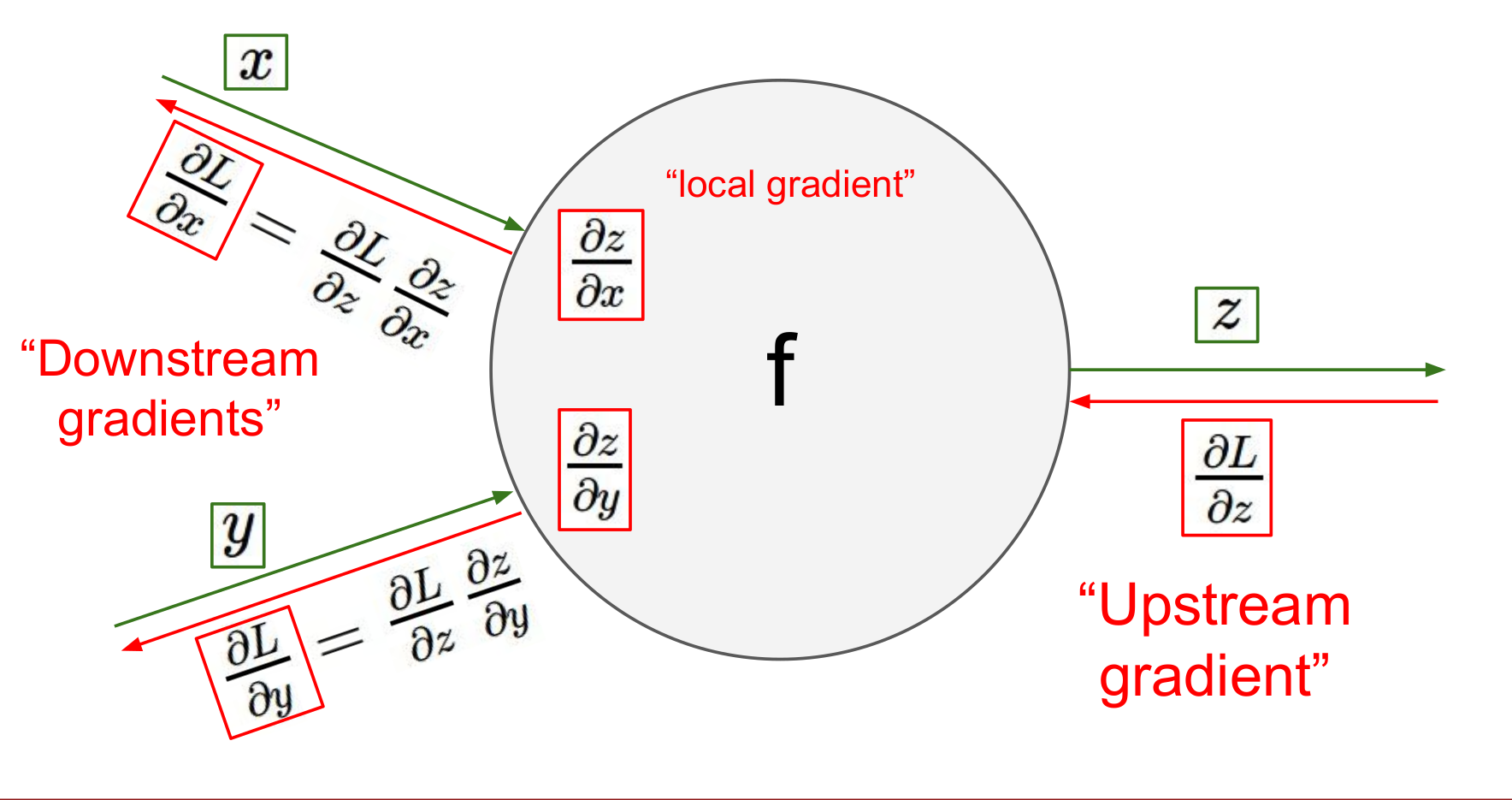
Gradient returned by the backward method of the class should have the same shape as the input to the forward method of the class, so that the gradient computed for the input after the loss.backward() step has the same shape as input and can be used to update it in the optimizer.step()
loss.backward() computes d(loss)/d(w) for every parameter which has requires_grad=True. They are accumulated in w.grad. And the optimizer.step() updates w using w.grad, w += -lr* x.grad
For more info read the posts below
Avoid using in-place operations as they cause problems while back-propagation because of the way they modify the graph. As a precaution, always clone the input in the forward pass, and clone the incoming gradients before modifying them.
An in-place operation directly modifies the content of a given Tensor without making a copy. Inplace operations in PyTorch are always postfixed with a , like .add() or .scatter_(). Python operations like + = or *= are also in-place operations.
Dealing with non-differentiable functions
Sometimes in your model or loss calculation you need to use functions that are non-differentiable. For calculating gradients, autograd requires all components of the graph to be differentiable. You can work around this by using a proxy function in the backward pass calculations.
f_hard : non-differentiable
f_soft : differentiable proxy for w_hard
f_out = f_soft + (f_hard - f_soft).detach()  # in PyTorch
f_out = f_soft + tf.stop_grad(f_hard - f_soft) # in Tensorflow
Core Idea
y = x_backward + (x_forward - x_backward).detach()It gets you x_forward in the forward pass, but derivative acts as if you had x_backward
class Binarizer(torch.autograd.Function):
    """
    An elementwise function that bins values
    to 0 or 1 depending on a threshold of 0.5,
    but in backward pass acts as an identity layer.

    Such layers are also known as
    straight-through gradient estimators

    Input: a tensor with values in range (0,1)
    Returns: a tensor with binary values: 0 or 1
    based on a threshold of 0.5
    Equation(1) in paper
    """
    @staticmethod
    def forward(ctx, i):
        return (i>0.5).float()

    @staticmethod
    def backward(ctx, grad_output):
        return grad_output

def bin_values(x):
    return Binarizer.apply(x)
The above function can be reimplemented with a single line in Pytorch while maintaining differentiabilty
def bin_values(x):
    return x + ((x>0.5).float() - x).detach()
Basic Training and Validation Loop
def fit(epochs, model, loss_func, opt, train_dl, valid_dl):
    for epoch in range(epochs):
        # Handle batchnorm / dropout
        model.train()
        # print(model.training)
        for mini_batch in train_dl:
            pred = model(mini_batch)
            loss = loss_func(pred, target)
            loss.backward()
            optimizer.step()
            optimizer.zero_grad()

        model.eval()
        #print(model.training)
        with torch.no_grad():
            for mini_batch in valid_dl:
                pred = model(mini_batch)
                # log some metrics here
            # aggregate metrics from all batches
Once you become more familiar with writing training and validation loops, I would recommend you to try out PyTorch Lightning PyTorch Lightning , which is a great library started by William Falcon that helps you get rid of all the PyTorch boilerplate code and instead lets you focus on the research part of your project.
Creating a SummaryWriter
from torch.utils.tensorboard import SummaryWriter
writer_train = SummaryWriter(os.path.join(args.experiment_dir,"tensorboard"))
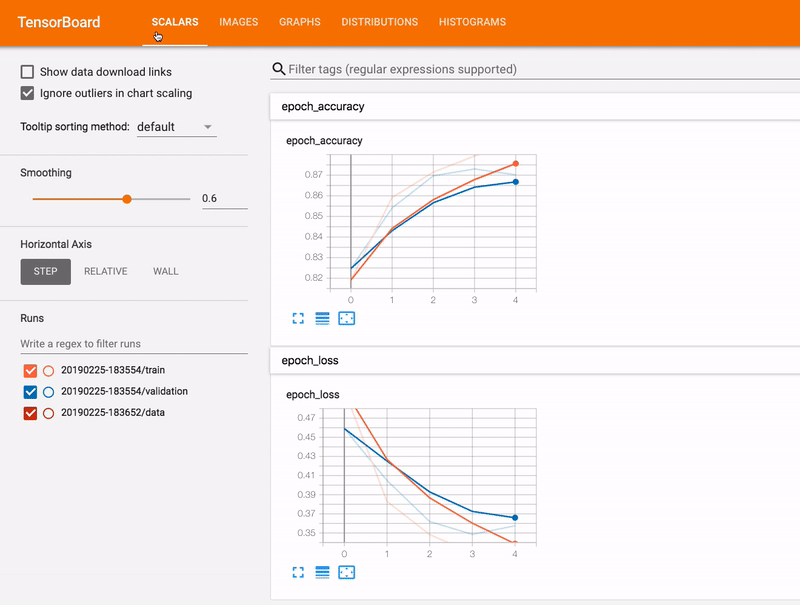
Scalars
Logging statements are added at different steps in the training loop wherever you want to log something. You can track scalars, images and even histograms. You can read more about this on the official PyTorch docs
Logging scalars can be as simple as
writer_train.add_scalar('train_loss', loss.item(), iteration)
where iteration is the global_step_count that you can keep track of inside your training loop.
Images
We'll use make_grid to create a grid of images directly from tensors so that we can plot them together.
from torchvision.utils import make_grid

# x is a tensor of Images of the shape (N,3,H,W)
x_grid = make_grid(x[:5],nrow=5)
writer_train.add_image('train/original_images',x_grid, iteration)
Launch
To visualize what you've logged, launch a tensorboard instance from the terminal by entering tensorboard --logdir . in the directory where you have logged your experiments.
Inference
To make predictions out of your trained model, make sure you feed data in the right format.
Input Tensor Format : (batch_size, channels, height, width). The model and the convolutional layers expect the input tensor to be of the shape (N,C,H,W), so when feeding an image/images to the model, add a dimension for batching.
Converting from img-->numpy representation and feeding the model gives an error because the input is in ByteTensor format. Only float operations are supported for conv-like operations. So add an extra step after numpy conversion -
img = img.type('torch.DoubleTensor')
Saving and Loading Models
PyTorch saves a model as a state_dict and the extension used is .pt
torch.save(model.state_dict(), PATH = 'latest_checkpoint.pt')
Sometimes you add new layers to your model which which were not present in the model you saved as checkpoint. In such a case set the strict keyword to False
model = Model()
checkpoint = torch.load('latest_checkpoint.pt')
model.load_state_dict(checkpoint, strict=False)
On Loading a model, if it shows a message like this, it means there were no missing keys and everything went well ( it's not an error ).
IncompatibleKeys(missing_keys=[], unexpected_keys=[])Keyboard interrupt and saving the last state of a model if you need to stop the experiment mid-way of training:
try:
    # training code here
except KeyboardInterrupt:
    # save model here
Extra Resources
- Grokking PyTorch
- Effective PyTorch
- The Python Magic Behind PyTorch
- Python is Cool - ChipHuyen
- PyTorch StyleGuide
- Clean Code Python
- Using _ in Variable Naming
- Pytorch Coding Conventions
- Fine Tuning etc
- https://github.com/dsgiitr/d2l-pytorch
- https://github.com/L1aoXingyu/pytorch-beginner
- https://github.com/yunjey/pytorch-tutorial
- https://github.com/MorvanZhou/PyTorch-Tutorial